Reinforcement Learning for LLMs

1. Basics

• RLHF: Reinforcement Learning from Human Feedback
• SFT: Supervised Fine-Tuning

RL trains neural networks through trial and error. When finetuning a language model with RLHF, the model produces some text then receives a score/reward from a human annotator that captures the quality of that text. Then, we use RL to finetune the language model to generate outputs with high scores.

In this case, we cannot apply a loss function that trains the language model to maximize human preferences with supervised learning. This is because there’s no easy way to explain the score human give or connect it mathematically to the output of the neural network. In other words, we cannot backpropagate a loss applied to this score through the rest of the neural network. This would require that we are able to differentiate (i.e., compute the gradient of) the system that generates the score, which is a human that subjectively evaluates the generated text.

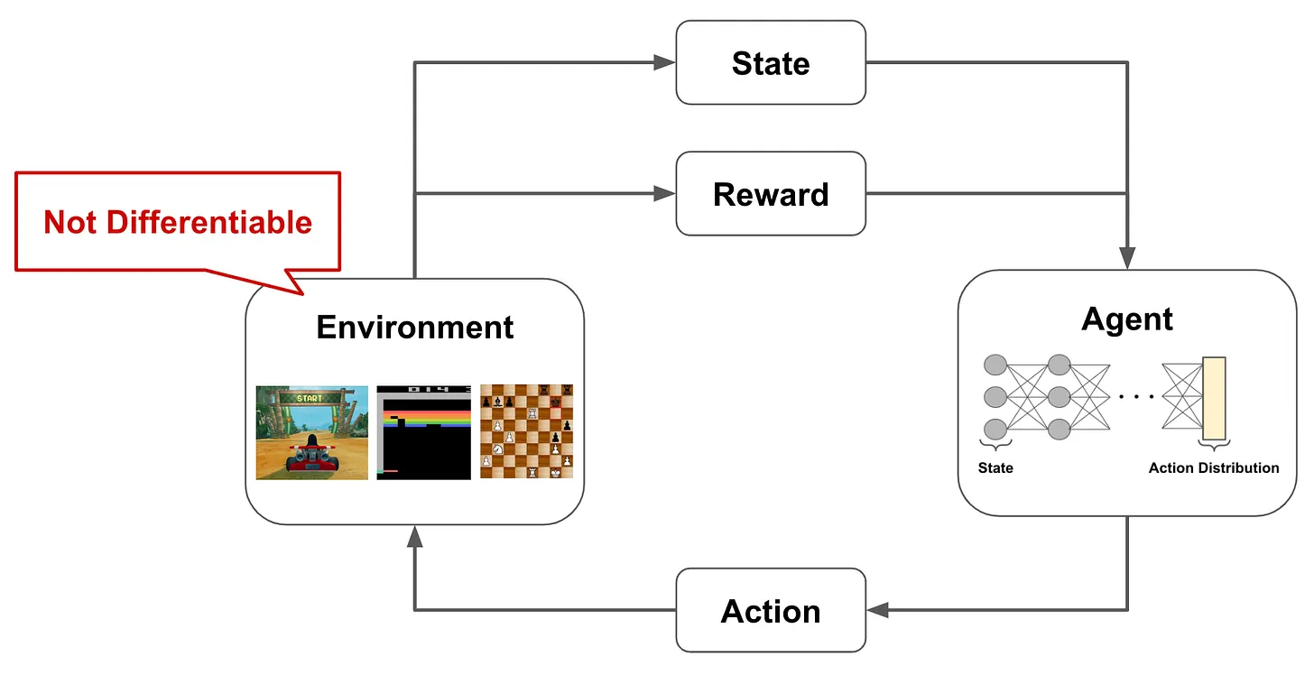
Problems that are solved via RL tend to be structured in a similar format. Namely, we have an agent that is interacting with an environment; see the figure above. The agent has a state in the environment and produces actions, which can modify the current state, as output. As the agent interacts with the environment, it can receive both positive and negative rewards for its actions. The agent’s goal is to maximize the rewards that it receives, but there is not a reward associated with every action taken by the agent. Rather, rewards may have a long horizon, meaning that it takes several correct, consecutive actions to generate any positive reward.

2. Markov Decision Process (MDP)

2.1. Concepts and Definitions

Markov Decision Process (MDP) is a way to formulate the system described above more formally and mathematically. Within an MDP, we have states, actions, rewards, transitions, and a policy, as shown in the equation below:

$$ \begin{cases} s \in S & \text{State} \\ a \in A & \text{Action} \\ r_s \in \mathbb{R} & \text{Reward} \\ \pi(a|s) & \text{Policy} \\ T(s_{t+1}|s_{t},a_{t}) & \text{Transition function} \\ \end{cases} $$

States and actions have discrete values, while rewards are real numbers.

In an MDP, we define two types of functions: transition and policy functions. The policy takes a state as input, then outputs a probability distribution over possible actions.

Notably, the action that is chosen only depends on the current state and not any state history that precedes it. This is a key property of an MDP, which make the assumption that the next action only depends upon the current state.

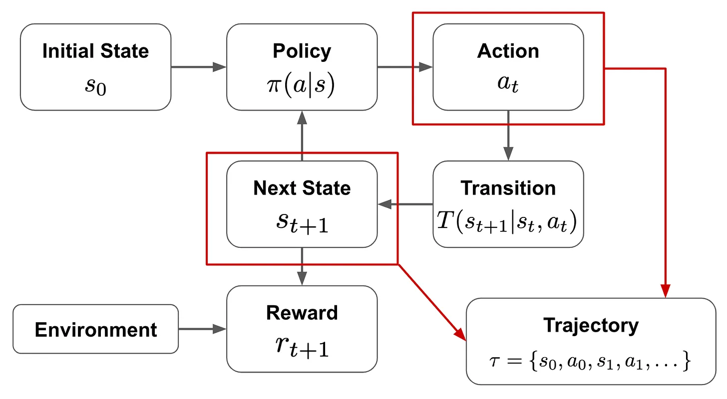
Given this output, we can make a decision for the action to be taken from a current state, and the transition is then a function that outputs the next state based upon the prior state and chosen action. Using these components, the agent can interact with the environment in an iterative fashion, as the figure shown below.

• The policy describes how the agent chooses its next action given the current state.
• The agent follows this strategy as it interacts with the environment.
• The goal is to learn a policy that maximizes the reward that the agent receives from the environment.

As the agent interacts with the environment, we form a trajectory ($\tau$) of states ($s$) and actions ($a$) that are chosen throughout this process. Then, given the reward ($r_s$) associated with each of these states, we get a total return ($R(\tau)$) given by the equation below, where $\gamma$ is the discount factor:

$$ \begin{cases} \tau &= \{s_0, a_0, s_1, a_1, \dots, s_t, a_t\} \quad &\text{(Trajectory)} \\ R(\tau) &= \sum_t \gamma^t r_{s_t} \quad &\text{(Return)} \end{cases} $$

$R(\tau)$ is the summed reward across the agent’s full trajectory, but rewards achieved at later time steps are exponentially discounted by the factor $\gamma$ TL;DR. The fact that the discount rate is bounded to be smaller than 1 is a mathematical trick to make an infinite sum finite. This helps proving the convergence of certain algorithms. See Understanding the role of the discount factor in reinforcement learning. — This means that current rewards are more valuable than later rewards, due to both uncertainty and the simple fact that waiting to receive a reward is less desirable.

The goal of RL is to train an agent that maximizes this return. As shown by the equation below, we can characterize this as finding a policy that maximizes the return over trajectories that are sampled from the final policy:

Note that the policy is a probability distribution over actions at each time step given the current state, so the exact trajectory produced is not deterministic. Many different trajectories can be obtained depending upon how we sample actions from the policy.

$$ \max_{\pi} ~ \mathbb{E}_{\tau \sim P_{\pi, T}} ~ R(\tau) $$

where:

• $\max_{\pi}$ means to find the policy that yields the maximum return.
• $\mathbb{E}_{\tau \sim P_{\pi, T}}$ means to take the expectation or average over trajectories randomly sampled from a certain policy $\pi$ and transition function $T$.
• $R(\tau)$ is the return of the trajectory $\tau$.

2.2. A Classical Example

A classical example of an MDP is a maze, where the agent is trying to find the optimal path to the goal.

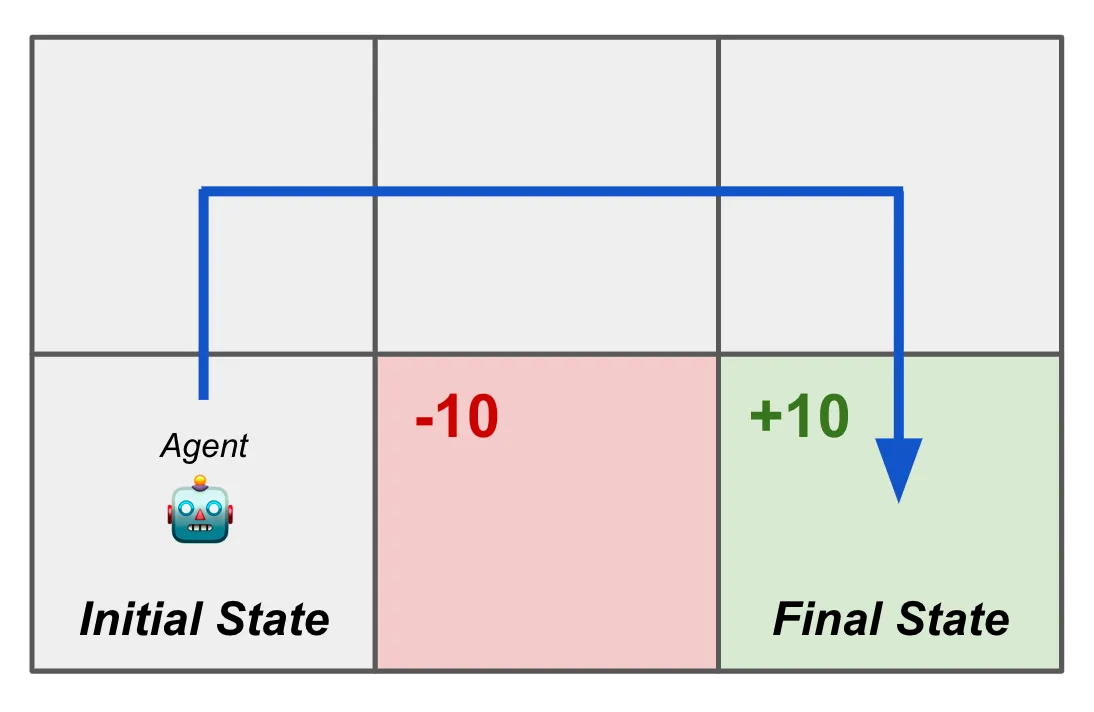
• States: The positions in the $2 \times 3$ maze. The positions can be represented as a one-hot vector.
• Actions: The possible moves (up, down, left, right) — This is the agent’s (i.e., the model’s) each-step output.
• Rewards: The agent receives a reward of $+10$ for reaching the goal and $-10$ for reaching the trap. The agent receives a reward of $0$ for all other states.
• Transition function: The agent can move to an adjacent state based on the chosen action, but it cannot move through walls. The transition function defines how the agent moves from one state to another based on the action taken.
• Policy: The agent’s policy is a probability distribution over the possible actions given the current state. For example, if the agent is in the state (0, 0), it might have a policy that gives a high probability to moving right and a low probability to moving down.
• Trajectory: The sequence of states and actions taken by the agent as it navigates the maze.

Like many problems that are solved with RL, this setup has an environment that is not differentiable (i.e., we can’t compute a gradient and train the model in a supervised fashion) and contains long-term dependencies, meaning that we might have to learn how to perform several sequential actions to get any reward.

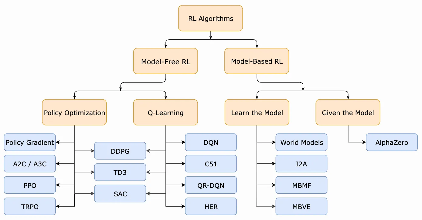
2.3. Taxonomy of modern RL algorithms

3. Deep Q-Leanring

3.1. Q-Learning

Q-Learning is a model-free RL algorithm, meaning that we don’t have to learn a model for the environment with which the agent interacts. The goal of Q-Learning is to learn the value of any action at a particular state.

There are three key concepts to mention here:

1. Value $Q(s, a)$ corresponds to choosing action $a$ at current state $s$. The value not only contains the determined reward by taking action $a$ at state $s$, but also contains a discounted and recursive future Q-value of the next state $s'$ after taking action $max_a$ (i.e., the best action at state $s'$).
2. The higher a value $Q(s, a)$ is, the more valuable it is to take action $a$ at state $s$.
3. A look-up table (Q-table) must be maintained to store the Q values for each state-action pair.

The algorithm first initialize all Q values as zero and pick an initial state with which to start the learning process. Then, iterate over the following steps:

• Pick an action to execute from the current state (using an $\varepsilon$-Greedy Policy).
• Get a reward and next state from the (model-free) environment.
• Update the Q value in the Q-table based on the Bellman equation.

Here we show a simplified update method which derives from the Bellman Optimality Equation and defines $Q(s_t, a_t)$ recursively:

$$ Q(s_t, a_t) = r_t + \gamma \max_{a} Q(s_{t+1}, a) $$

where:

• $Q(s_t, a_t)$ is the Q value of the current state $s_t$ and action $a_t$.
• $r_t$ is the reward received after taking action $a_t$ at state $s_t$.
• $\gamma$ is the discount factor.
• $\max_{a} Q(s_{t+1}, a)$ is the maximum Q value of the next state $s_{t+1}$ over all possible actions $a$.

3.2. Deep Q-Learning (DQL)

In DQL, Q-table is replaced by a neural network.

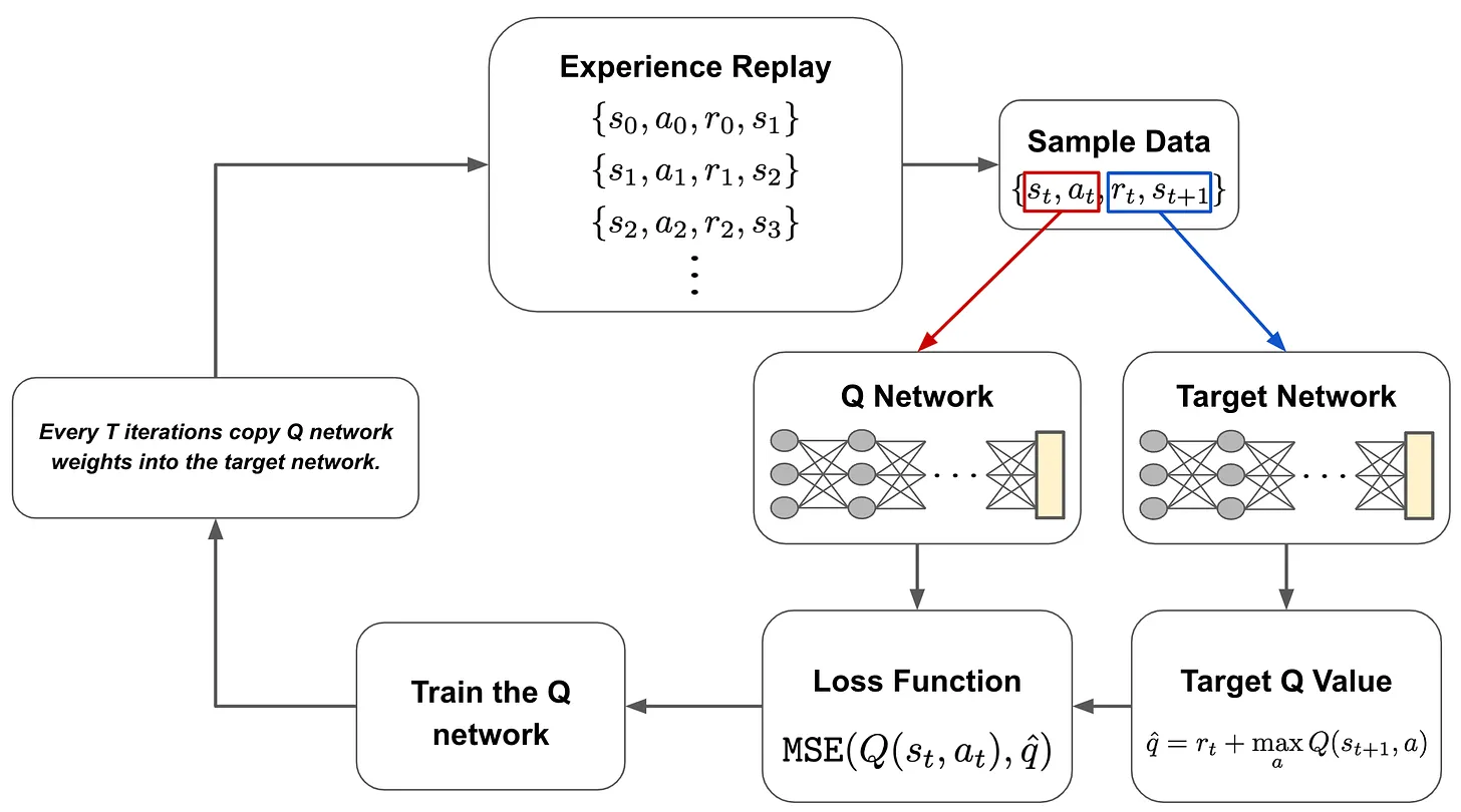
In DQL, we have two neural networks: the Q network and the target network. These networks are identical, but the exact architecture they use depend upon the problem being solved7. To train these networks, we first gather data by interacting with the environment. This data is gathered using the current Q network with an ε-greedy policy. This process of gathering interaction data for training the Q network is referred to as experience replay; see above.

From here, we use data that has been collected to train the Q network. During each training iteration, we sample a batch of data and pass it through both the Q network and the target network. The Q network takes the current state as input and predicts the Q value of the action that is taken (i.e., predicted Q value), while the target network takes the next state as input and predicts the Q value of the best action that can be taken from that state8 (i.e., target Q value).

From here, we use the predicted Q value, the target Q value, and the observed reward to train the Q network with an MSE loss; see above. The target network is held fixed. Every several iterations, the weights of the Q network are copied to the target network, allowing this model to be updated as well. Then, we just repeat this process until the Q network converges. Notably, the dataset we obtain from experience replay is cumulative, meaning that we maintain all of the data we have observed from the environment throughout all iterations.

Why do we need the target network? The vanilla Q-learning framework leverages two Q values in its update rule: a (predicted) Q value for the current state-action pair and the (target) Q value of the best state-action pair for the next state. In DQL, we similarly have to generate both of these Q values. In theory, we could do this with a single neural network by making multiple passes through the Q network—one for the predicted Q value and one for the target Q value. However, the Q network’s weights are being updated at every training iteration, which would cause the target Q value to constantly fluctuate as the model is updated. To avoid this issue, we keep the target network separate and fixed, only updating its weights every several iterations to avoid creating a “moving target”.

This idea of using a separate network to produce a training target for another network—referred to as knowledge distillation [6]—is heavily utilized within deep learning. Furthermore, the idea of avoiding too much fluctuation in the weights of the teacher/target model has been addressed in this domain. For example, the mean teacher approach [7] updates the weights of the teacher model as an exponential moving average of the student network’s weights; see above. In this way, we can ensure a stable target is provided by the teacher during training.

4. Policy Gradients

In Policy Gradients, we will assume that our policy is a machine learning model (e.g., a deep neural network) with parameters $\theta$. This policy takes a state as input and predicts some distribution over the action space. We use this output to decide what action should be taken next within the MDP:

$$ \begin{cases} s \in S & \text{State} \\ a \in A & \text{Action} \\ r_s \in \mathbb{R} & \text{Reward} \\ \pi_{\theta}(a|s) & \text{Policy} \\ T(s_{t+1}|s_{t},a_{t}) & \text{Transition function} \\ \end{cases} $$

As our agent traverses the environment, it receives positive or negative reward signals for the actions it chooses and the states that it visits. Our goal is to learn a policy from these reward signals that maximizes total reward across an entire trajectory sampled from the policy. This idea is captured by the return, which sums the total rewards over an agent’s trajectory:

$$ \begin{cases} \tau &= \{s_0, a_0, s_1, a_1, \dots, s_t, a_t\} \quad &\text{(Trajectory)} \\ R(\tau) &= \sum_t \gamma^t r_{s_t} \quad &\text{(Return)} \end{cases} $$

If $\gamma < 1$, then the return is Infinite-Horizon Discounted Return. If $\gamma = 1$, then the return is Finite-Horizon Return.

4.1. Value Functions and Advantage Functions

One final concept that will be especially relevant is that value functions. In RL, there are four basic value functions, all of which assume the infinite-horizon discounted return:

$$ \begin{align*} V^{\pi}(s) &= \mathbb{E}_{\tau \sim (\pi,T)} [R(\tau)|s_0 = s] && \text{(On-Policy Value Function)} \\ Q^{\pi}(s, a) &= \mathbb{E}_{\tau \sim (\pi,T)} [R(\tau)|s_0 = s, a_0 = a] && \text{(On-Policy Action-Value Function)} \\ V^{*}(s) &= \max_{\pi} \mathbb{E}_{\tau \sim (\pi,T)} [R(\tau)|s_0 = s] && \text{(Optimal Value Function)} \\ Q^{*}(s, a) &= \max_{\pi} \mathbb{E}_{\tau \sim (\pi,T)} [R(\tau)|s_0 = s, a_0 = a] && \text{(Optimal Action-Value Function)} \end{align*} $$

• On-Policy Value Functio: expected return if starting in state $s$ and act according to policy $\pi$ afterwards.
• On-Policy Action-Value Function: expected return if you start in state $s$, take some action $a$ (may not come from the current policy), and act according to policy $\pi$ afterwards.
• Optimal Value Function: expected return if you start in state $s$ and always act according to the optimal policy afterwards.
• Optimal Action-Value Function: expected return if you start in state $s$, take some action a (may not come from the current policy), and act according to the optimal policy afterwards.

There is an important connection between the optimal policy in an environment and the optimal action-value function. Namely, the optimal policy selects the action in state $s$ that maximizes the value of the optimal action-value function.

Using the value functions described above, we can define a special type of function called an advantage function, which is heavily used in RL algorithms based on policy gradients:

$$ A^{\pi}(s, a) = Q^{\pi}(s, a) - V^{\pi}(s) \quad \text{(Advantage Function)} $$

• $Q^{\pi}(s, a)$ on-policy action-value function.
• $V^{\pi}(s)$ on-policy value function.

Simply put, the advantage function characterizes how much better it is to take a certain action a relative to a randomly-selected action in state $s$ given a policy $\pi$. Here, we should notice that the advantage function can be derived using the on-policy value and action-value functions defined before, as these functions assume that the agent acts according to a randomly-selected action from the policy $\pi$.

The value of your starting point is the reward you expect to get from being there, plus the value of wherever you land next. —— [3]

4.2. Policy Optimization

During the learning process, we aim to find parameters $\theta$ for our policy that maximize the objective function below:

$$ \mathcal{J}(\pi_{\theta}) = \mathbb{E}_{\tau \sim (\pi_{\theta},T)} [R(\tau)] $$

where:

• $\pi_{\theta}$ is the policy with network parameters $\theta$.
• $\tau$ is the trajectory sampled from the policy $\pi_{\theta}$ and transition function $T$.
• $T$ is the transition function that defines how the agent moves from one state to another based on the action taken.
• $R(\tau)$ is the return of the trajectory $\tau$.

In words, this objective function measures the expected return of trajectories sampled from our policy within the specified environment.

If we want to find parameters $\theta$ that maximize this objective function, one of the most fundamental techniques that we can use is gradient ascent, which iterates over parameters $\theta$ using the update rule shown below:

$$ \theta_{t+1} = \theta_t + \alpha \nabla_{\theta} \mathcal{J}(\pi_{\theta})|_{\theta_t} $$

Do a lot of math to compute $\nabla_{\theta} \mathcal{J}(\pi_{\theta})$, and the final result of the basic policy gradient is:

$$ \nabla_{\theta} \mathcal{J}(\pi_{\theta}) = \mathbb{E}_{\tau \sim (\pi_{\theta}, T)} \left[ \sum_{t=0}^{T} \nabla_{\theta} \log \pi_{\theta}(a_t|s_t) R(\tau) \right] $$

Now, we have an actual expression for the gradient of our objective function that we can use in gradient ascent! Plus, this expression only depends on the return of a trajectory and the gradient of the log probability of an action given our current state. As long as we instantiate our policy such that the gradient of action probabilities is computable (e.g., this is pretty easy to do if our policy is implemented as a neural network), we can easily derive both of these quantities.

4.3. Computing the Policy Gradient in Practice

In practice, we can estimate the value of this expectation by sampling a fixed number of trajectories, by:

• Sample several trajectories by letting the agent interact with the environment according to the current policy.
• Estimate the policy gradient using an average of relevant quantities over the fixed number of sample trajectories.

Then given a set of sampled trajectories $\mathcal{D} = \{\tau_0, \tau_1, \dots\}$, we can estimate the policy gradient $\overline{\nabla_{\theta} \mathcal{J}(\pi_{\theta})}$ as follows:

$$ \overline{\nabla_{\theta} \mathcal{J}(\pi_{\theta})} = \frac{1}{|\mathcal{D}|} \sum_{\tau \in \mathcal{D}} \sum_{t=0}^{T} \left[ \nabla_{\theta} \log \pi_{\theta}(a_t|s_t) R(\tau) \right] $$

4.4. Vallina Poclicy Gradient (VPG) and Other Policy Gradients

Given:

$$ \nabla_{\theta} \mathcal{J}(\pi_{\theta}) = \mathbb{E} \left[ \sum_{t=0}^{T} \nabla_{\theta} \log \pi_{\theta}(a_t|s_t) \Psi_t \right] $$

We have:

1. Basic Policy Gradient: $$ \Psi_t = R(\tau) $$ Sum of all (potentially discounted) rewards obtained along the entire trajectory.
2. Reward-to-Go: $$ \Psi_t = \sum_{i=t}^{T} r_{s_i, a_i} $$ Rewards after the current action.
3. Reward-to-Go with Baseline: $$ \Psi_t = \sum_{i=t}^{T} r_{s_i, a_i} - b(s_i) $$ A baseline function to our expression that only depends on the current state.
4. Vallina Policy Gradient (VPG): $$ \Psi_t = A^{\pi_{\theta}}(s_t, a_t) = Q^{\pi_{\theta}}(s_t, a_t) - V^{\pi_{\theta}}(s_t) $$ where $A^{\pi_{\theta}}(s_t, a_t)$ is the advantage function, $Q^{\pi_{\theta}}(s_t, a_t)$ is the action-value function, and $V^{\pi_{\theta}}(s_t)$ is the value function.

TODO: Why use VPG?

5. Proximal Policy Optimization (PPO)

• DQL: can only be applied in relatively simple environments.
• VPG: has poor data efficiency and robustness, meaning that we must collect tons of data from our environment to eliminate noise within the policy gradient estimate.

Motivation for TRPO and PPO:

• Generally applicable (i.e., to both discrete and continuous problems)
• Data efficient
• Robust (i.e., works without too much tuning)
• Simple (i.e., not too difficult to understand/implement)

TRPO satisfies the first two points outlined above, while PPO satisfies all four.

5.1. Aligning LLMs with RL

After pre-training, the model perfroms next token prediction, but its output may be repetitive, uninteresting, or not useful. That’s the reason alignment is needed.

Typically, we perform alignment by

1. Selecting several alignment criteria (e.g., follow instructions, avoid harmful output, avoid hallucination, produce interesting/creative output, etc.)
2. Finetuning the model —— via SFT and RLHF —— to satisfy these criteria.
3. The final model can further finetuned and used to solve a downstream application via prompting (or in-context learning).

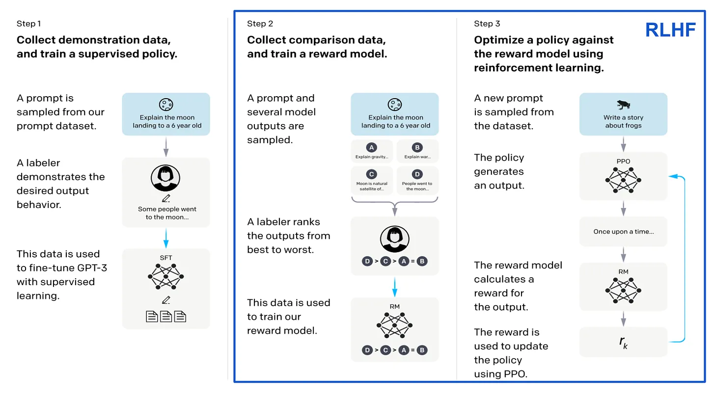
As shown in the figure above, to apply RLHF:

1. Prepare a set of prompts and generate several outputs for each prompt with the language model.
2. Ask a group of human annotators to rank/score the responses to each prompt according to our alignment criteria.
3. Use these ranked responses to train a reward model that predicts a human preference score from a language model’s response.
4. Use PPO (or other algorithms, e.g., VPG, TRPO) to finetune our language model to maximize the human preferences scores (predicted by the reward model) of its outputs.

5.2. Kullback–Leibler (KL) Divergence

At the highest level, the Kullback-Leibler (KL) Divergence is just a method of comparing two probability distributions.

The idea of KL divergence has its roots in information theory and is highly related to the concept of entropy According to Shannon’s Source Coding Theorem, the optimal number of bits required to encode a message with probability $p(x)$ is given by $−\log_{2}{p(x)}$.
High probability event ($p(x) \approx 1$): $−log_2​(1)=0$. It takes very few bits to encode a highly probable event.
Low probability event ($p(x) \approx 0$): $−log_2​(p(x))$ is a large number. It takes many bits to encode a rare event. :

$$ H= \begin{cases} -\mathbb{E} \left[ \log p(x) \right] &\text{(Continuous Case)} \\ -\sum_{i=1}^{N} p(x_i) \cdot \log p(x_i) &\text{(Discrete Case)} \end{cases} $$

In the equation above, we can see common formulations of entropy $H$ for a probability distribution $p$. Intuitively, the entropy value captures how much information is stored within a probability distribution —— a lower entropy means that you would need fewer bits to encode the information stored within $p$.

Instead of a single probability distribution $p$, the KL divergence considers two probability distributions: $p$ and $q$. Then, mirroring the above entropy formulation, we compute KL divergence by finding the expected difference in log probabilities between these two distributions:

$$ \begin{align*} D_{\text{KL}}(p||q) &= H(p, q) - H(p) \\ &= \begin{cases} \mathbb{E} \left[ \log p(x) - \log q(x) \right] ~~~ \text{(Continuous Case)} \\ \sum_{i=1}^{N} p(x_i) \cdot \left( \log p(x_i) - \log q(x_i) \right) ~~~ \text{(Discrete Case)} \end{cases} \end{align*} $$

where:

• $H(p,q)$: The average number of bits used with the approximate code.
• $H(p)$: The minimum possible average number of bits used with the optimal code.
• $D_{\text{KL}}(p||q)$: The penalty, or the expected number of extra bits “wasted” or “lost” per message due to the approximation.

The KL divergence is commonly explained in the context of approximations. Namely, if we approximate $p$ with $q$, the KL divergence is the number of bits we would expect to lose by making this approximation.

KL divergence is heavily used across different domains of AI/ML research. For example, it is commonly used in loss functions for training neural networks, either as the core loss or as an added regularization term.

The final reward function we use during optimization contains a [KL divergence] penalty term … we find this constraint is useful for training stability, and to reduce reward hacking.” —— [4]

5.3. Trust Region Policy Optimization (TRPO)

VPG is limited by the fact that it can only perform a single policy update for each estimate of the policy gradient that is derived. Given that VPG is notoriously data inefficient, meaning that we have to sample a lot of data when deriving a policy update, performing multiple (or larger) updates may seem enticing. However, such an approach is not justified theoretically and, in practice, leads to policy updates that are too large, thus damaging performance.

Trust Region Policy Optimization (TRPO) [5] aims to solve the problem described above using an approach that is similar to VPG. At each step of the optimization process, however, we find the largest possible policy update that still improves performance. Simply put, TRPO allows us to learn faster by finding a reliable way to make larger policy updates that do not damage performance.

More specifically, we update the policy under a constraint—based on the KL divergence—that captures the distance between policies before and after the current update. Considering this constraint allows us to find a balance between update size and the amount of change to the underlying policy:

$$ \begin{equation*} \begin{gathered} \theta_{k+1} = \operatorname{argmax}_{\theta} \mathbb{E}_{(s,a) \sim (\pi_{\theta_k}, T)} \left[ \frac{\pi_{\theta}(a|s)}{\pi_{\theta_k}(a|s)} A^{\pi_{\theta_k}}(s,a) \right] \\ \text{such that } \overline{D}_{\text{KL}}(\theta||\theta_k) < \delta \end{gathered} \end{equation*} $$

where:

• $\mathbb{E}_{(s,a) \sim (\pi_{\theta_k}, T)}$ is the expectation over state-action pairs sampled from the current policy $\pi_{\theta_k}$ and transition function $T$.
• $\pi_{\theta}(a|s)$ is the probability of taking action $a$ in state $s$ according to the new policy $\pi_{\theta}$.
• $\pi_{\theta_k}(a|s)$ is the probability of taking action $a$ in state $s$ according to the current policy $\pi_{\theta_k}$.
• $A^{\pi_{\theta_k}}(s,a)$ is the advantage function for the current policy $\pi_{\theta_k}$.
• $\overline{D}_{\text{KL}}(\theta||\theta_k)$ is the average KL divergence between the new policy $\pi_{\theta}$ and the current policy $\pi_{\theta_k}$.
• $\delta$ is a hyperparameter that controls the maximum allowed change in the policy.

Formulation of TRPO has several critical differences from VPG:

• The terms in the expectation are modified slightly to express the probability of a given action a as a ratio between old and updated policies.
• The update has an added constraint based on the KL divergence between old and updated policies.
• Instead of performing gradient ascent, we are solving a constrained maximization problem to generate each new policy

The implementation of TRPO is similar to that of VPG. We allow our current policy to interact with the environment and collect data. From this observed data, we can compute the approximate update for TRPO as described above. Then, we can continue the process of collecting data and performing an update until we arrive at a policy that performs quite well.

Because we are using the actual policy being trained to collect the data used to train it, TRPO is an on-policy reinforcement learning algorithm.

5.4. TRPO vs. VPG: Larger Policy Updates

As mentioned previously, the VPG algorithm is based upon gradient ascent, which —— by nature —— ensures that updates to the policy’s parameters $\theta$ are not too large. In particular, we use a learning rate to perform updates with VPG, which can control the size of the update in the parameter space:

$$ \theta_{t+1} = \theta_t + \alpha \nabla_{\theta} J(\pi_{\theta})|_{\theta_t} $$

Here, only the size of the update to $\theta$ is controlled, and so that the old and updated policies are close in the parameter space. However, small changes to $\theta$ may also drastically alter the policy, because ensuring that policy updates are small in the parameter space does not provide much of a guarantee on changes to the resulting policy.

As a result, we are constrained to relatively small updates within the VPG algorithm —— larger or multiple updates could be harmful.

TRPO sidesteps this issue by considering the size of our policy update from an alternative viewpoint. Namely, we compare updated and old policies using the KL divergence, which measures the difference in probability distributions over the action space produced by the two policies. Such an approach compares policies based upon the actions they take rather than their underlying parameters $\theta$.

In this way, we can perform large policy updates while ensuring that the new policy does not produce actions that are significantly different from the old policy.

5.5. Proximal Policy Optimization (PPO)

We introduce proximal policy optimization, a family of policy optimization methods that use multiple epochs of stochastic gradient ascent to perform each policy update. These methods have the stability and reliability of trust-region methods but are much simpler to implement … applicable in more general settings, and have better overall performance. —— [6]

TRPO has improved data efficiency, stability, and reliability compared to the VPG algorithm, but there are still limitations that need to be addressed.

Namely, the algorithm is complicated, can only perform a single update each time new data is sampled from the environment, and is only applicable to certain problem setups.

Aiming to develop a better approach, authors in [6] propose Proximal Policy Optimization (PPO), another policy gradient algorithm that alternates between collecting data from the environment and performing several epochs of training over this sampled data. PPO shares the reliability of TRPO and is:

1. Much simpler
2. More data efficient
3. More generally applicable

Similar to TRPO, we perform policy updates in PPO according to a surrogate objective. However, this surrogate objective has a “clipped” probability ratio, as shown in the equation below:

$$ L^{\text{CLIP}}(\theta) = \mathbb{E}_t \left[ \min(\frac{\pi_{\theta}(o_t|q, o_{< t})}{\pi_{\theta_{old}}(o_t|q, o_{< t})}A_t, \text{CLIP}(\frac{\pi_{\theta}(o_t|q, o_{< t})}{\pi_{\theta_{old}}(o_t|q, o_{< t})}, 1-\varepsilon, 1+\varepsilon) A_t) \right] $$

The surrogate objective for PPO is expressed as a minimum of two values. The first value is the same surrogate objective from TRPO, while the second value is a “clipped” version of this objective that lies within a certain range. In practice, this expression is formulated such that there is no reward for moving the probability ratio beyond the interval $[1 - \varepsilon, 1 + \varepsilon]$, see the figure below:

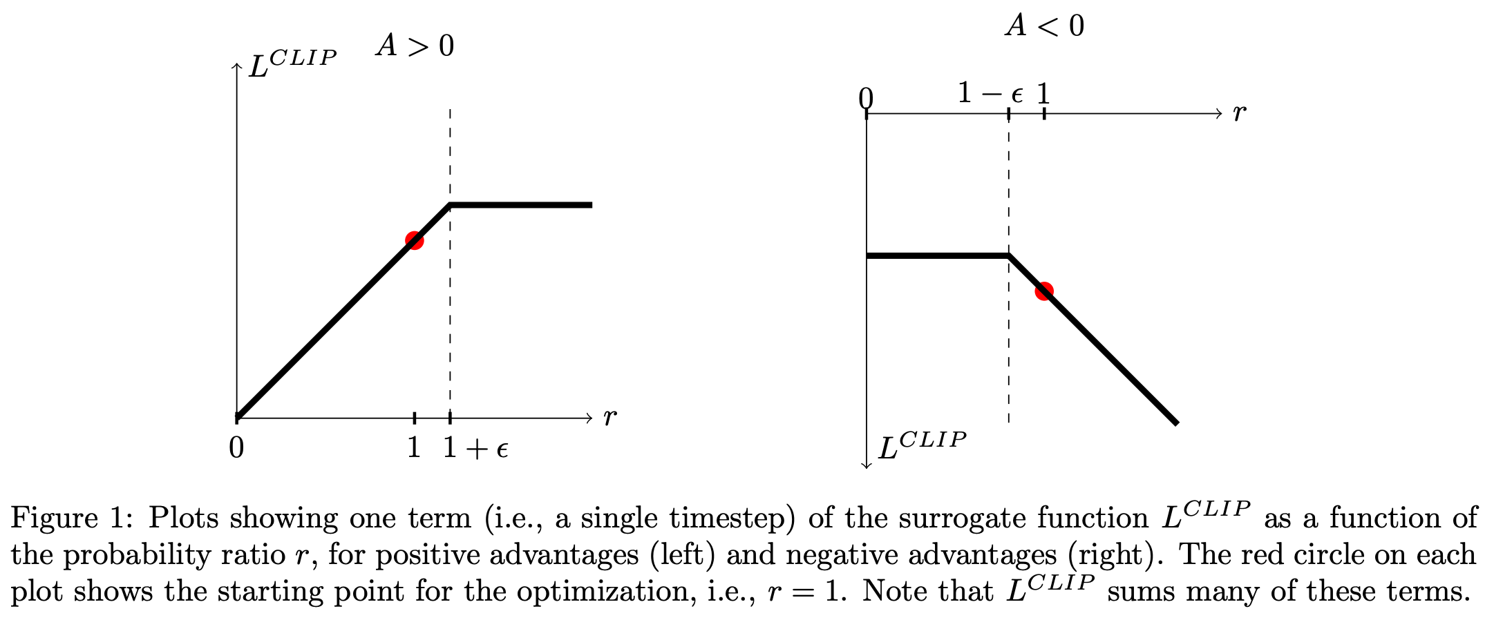
In other words, PPO has no incentive for excessively large policy updates. Plus, by taking the minimum of the clipped and unclipped version of the surrogate objective, we only ignore excessive changes to the probability ratio if they improve the underlying objective. In the figure above, we see a basic depiction of this trend for both positive and negative values of the advantage function.

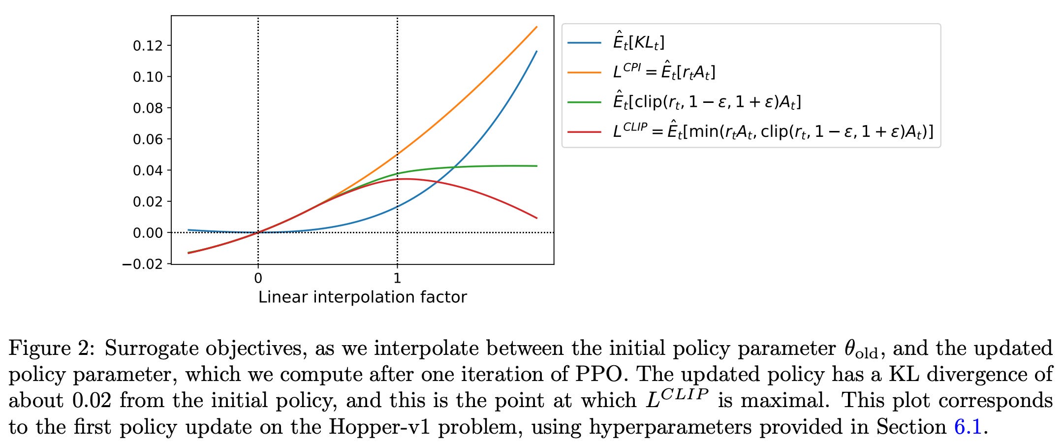
To understand PPO’s surrogate objective more intuitively, we should look at the figure below, which plots several objective functions as we interpolate between an old and updated policy obtained via PPO. In this figure, we see the KL divergence, the TRPO surrogate objective (labeled as CPI), the clipped surrogate objective, and the full PPO surrogate objective. From these plots, we can see that the PPO surrogate objective is a pessimistic/lower bound for the TRPO surrogate objective, where a penalty is incurred for having too large of a policy update.

While TRPO sets a hard constraint to avoid policy updates that are too large, PPO simply formulates the surrogate objective such that a penalty is incurred if the KL divergence is too large. Such an approach is much simpler, as we no longer have to solve a difficult, constrained optimization problem. Rather, we can compute PPO’s surrogate loss with only minor tweaks to the VPG algorithm.

PPO has several benefits compared to TRPO. First, the implementation of PPO is much simpler compared to TRPO, as we can use automatic differentiation and gradient-based optimization techniques9 instead of deriving an (approximate) solution for a complex, constrained objective function. Additionally, while TRPO makes only a single policy update each time new data is collected, PPO performs multiple epochs of optimization via stochastic gradient ascent over the surrogate objective, which improves data efficiency.

Finally, computing estimates of the advantage function (e.g., via Generalized Advantage Estimation (GAE)) typically requires that we learn a corresponding value function. In TRPO, we must learn this state-value function with a separate neural network. However, PPO—due to its compatibility with a wider scope of architectures (including those with parameter sharing) —— can train a joint network for policy and value functions by just adding an extra term to the loss function that computes the mean-squared error (MSE) between estimated and actual value function values.

$$ L^{\text{CLIP+VF}}(\theta) = \mathbb{E}_t \left[ L^{\text{CLIP}}(\theta) - c_1 L^{\text{VF}}(\theta) \right] $$

where:

• $L^{\text{CLIP}}(\theta)$ is the PPO surrogate objective.
• $L^{\text{VF}}(\theta)$ is the MSE loss for the value function.
• $c_1$ is a hyperparameter that controls the weight of the value function loss in the overall loss function.

6. Group Relative Policy Optimization (GRPO)

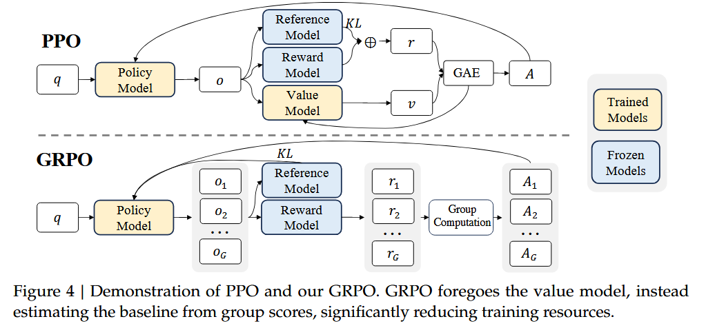
Different from PPO, GRPO:

1. Removes the value function model.
2. The policy model generates multiple outputs for each input, and the reward model calculates the reward for each output, and calculates the advantage scores after group computation.
3. Removes the GAE, and changes the method to calculate KL.

In PPO, we optimizes LLMs by maximizing the following objective function:

$$ \begin{align*} \mathcal{J}_{\text{PPO}}(\theta) = \mathbb{E}&_{q \sim P(Q), o \sim \pi_{\theta_{\text{old}}}(O|q)} \left[ \frac{1}{|o|} \sum_{t=1}^{|o|} \min \left( \frac{\pi_{\theta}(o_t|q, o_{< t})}{\pi_{\theta_{\text{old}}}(o_t|q, o_{< t})} A_t, \right. \right. \\ & \left. \left. \text{clip}\left(\frac{\pi_{\theta}(o_t|q, o_{< t})}{\pi_{\theta_{\text{old}}}(o_t|q, o_{< t})}, 1-\varepsilon, 1+\varepsilon\right) A_t \right) \right] \end{align*} $$

where:

• $\pi_{\theta}$ and $\pi{\theta_{\text{old}}}$ are the current and old policy models;
• $q$, $o$ are questions and outputs sampled from the question dataset and the old policy $\pi{\theta_{\text{old}}}$;
• $\varepsilon$ is a clipping-related hyper-parameter introduced in PPO for stabilizing training;
• $A_t$ is the advantage, which is computed by applying Generalized Advantage Estimation (GAE), based on the rewards ${r_{\geq t}}$ and a learned value function $V_{\psi}$.

Thus, in PPO, a value function needs to be trained alongside the policy model and to mitigate over-optimization of the reward model, the standard approach is to add a per-token KL penalty from a reference model in the reward at each token, i.e.:

$$ r_t = r_{\varphi}(q, o_{\leq t}) - \beta \log \frac{\pi_{\theta}(o_t|q, o_{< t})}{\pi_{ref}(o_t|q, o_{< t})} $$

There are several issues with PPO:

1. As the value function employed in PPO is typically another model of comparable size as the policy model, it brings a substantial memory and computational burden.
2. During RL training, the value function is treated as a baseline in the calculation of the advantage for variance reduction. While in the LLM context, usually only the last token is assigned a reward score by the reward model, which may complicate the training of a value function that is accurate at each token.

To address these issues, for each question $q$, GRPO samples a group of outputs $\{o_1, o_2, \dots , o_G\}$ from the old policy $\pi_{\theta_{\text{old}}}$ and then optimizes the policy model by maximizing the following objective:

$$ \begin{align*} \mathcal{J}_{\text{GRPO}}(\theta) = \mathbb{E}&[q \sim P(Q), \{o_i\}_{i=1}^G \sim \pi_{\theta_{\text{old}}}(O|q)] \\ &\frac{1}{G} \sum_{i=1}^G \frac{1}{|o_i|} \sum_{t=1}^{|o_i|} \left\{ \min\left(\frac{\pi_{\theta}(o_{i,t}|q, o_{i,< t})}{\pi_{\theta_{\text{old}}}(o_{i,t}|q, o_{i,< t})} \hat{A}_{i,t}, \right.\right. \\ &\left.\left. \text{clip}\left(\frac{\pi_{\theta}(o_{i,t}|q, o_{i,< t})}{\pi_{\theta_{\text{old}}}(o_{i,t}|q, o_{i,< t})}, 1-\varepsilon, 1+\varepsilon\right) \hat{A}_{i,t}\right) - \beta D_{KL}[\pi_{\theta}||\pi_{ref}] \right\} \end{align*} $$

where:

• $\varepsilon$ and $\beta$ are hyper-parameters;
• $\hat{A}_{i,t}$ is the advantage calculated based on relative rewards of the outputs inside each group only.

Note that:

1. Instead of adding KL penalty in the reward, GRPO regularizes by directly adding the KL divergence between the trained policy and the reference policy to the loss, avoiding complicating the calculation of $\hat{A}_{i,t}$.
2. Different from the KL penalty term used in [6], GRPO estimate the KL divergence with the following unbiased estimator: $$ \mathbb{D}_{\text{KL}}\left[ \pi_{\theta}||\pi_{ref}\right] = \frac{\pi_{ref}(o_{t,t}|q, o_{t,< t})}{\pi_{\theta}(o_{t,t}|q, o_{t,< t})} - \log \frac{\pi_{ref}(o_{t,t}|q, o_{t,< t})}{\pi_{\theta}(o_{t,t}|q, o_{t,< t})} - 1 $$ which is guaranteed to be positive.

References

1. Cameron R. Wolfe. Basics of Reinforcement Learning for LLMs .
2. Cameron R. Wolfe. Proximal Policy Optimization (PPO): The Key to LLM Alignment
3. Achiam, Josh. Spinning Up in Deep RL . OpenAI, 2018.
4. Touvron, Hugo, et al. “Llama 2: Open foundation and fine-tuned chat models.” arXiv preprint arXiv:2307.09288 (2023).
5. Schulman, John, Sergey Levine, Pieter Abbeel, Michael Jordan, and Philipp Moritz. “Trust region policy optimization.” In International conference on machine learning, pp. 1889-1897. PMLR, 2015.
6. Schulman, John, Filip Wolski, Prafulla Dhariwal, Alec Radford, and Oleg Klimov. “Proximal policy optimization algorithms.” arXiv preprint arXiv:1707.06347 (2017).
7. Shao, Zhihong, Peiyi Wang, Qihao Zhu, Runxin Xu, Junxiao Song, Xiao Bi, Haowei Zhang et al. “Deepseekmath: Pushing the limits of mathematical reasoning in open language models.” arXiv preprint arXiv:2402.03300 (2024).